Stat Unit

There are four areas within the broad area of descriptive statistics. These broad areas include:

• Frequency Distributions (Unit 2)
• Measures of Central Tendency (Unit 3)
• Measures of Variability (Unit 4)
• Measures of Position (Unit 5)
• Measures of Central Tendency

Measures of Central Tendency describe or summarize the middle or center of a distribution. Or we might say that measures of central tendency describe or summarize the typical score within a distribution. In this unit, we will look at three measures of central tendency:

• Mode
• Median
• Mean

Let's take a close look at each.

The mode is defined as the most frequently occurring score within a distribution. We could also define the mode as the score in a distribution that occurs most often. Consider the following example:

n the above distribution of five data values, the mode is 4 because 4 occurs twice and all other numbers occur only once each. Now let's alter the distribution:

The second distribution has two 3s and two 4s -- or two modes. Hence, this distribution is described as bi-modal.

A distribution may also be tri-modal (having three modes) or even multi-modal (having more than three modes).

Additionally, a distribution will not have a mode if every data value occurs once and only once:

The median is defined as the middle score in a ranked distribution of scores. The median is equal to or smaller than half of the terms in a distribution and equal to or larger than half the terms in a distribution. Consider the following distribution of five scores:

In this distribution of five data values, the median is 3 as 3 is the score that divides the distribution into two equal halves. There are two scores above the value 3 (1 and 2) and two scores below the value 3 (4 and 5).

Notice that this distribution has an odd number of scores (i.e., 5 scores).

How would calculation of the median change if the distribution had 6 scores or an even number of scores? When a distribution has an even number of scores, there is no true or actual median. In other words, there is no data value that is larger than half of the distribution and smaller than half of the distribution.

When a distribution has an even number of scores, the median is defined as the average of the two middle scores once the distribution is ranked. Consider the following example:

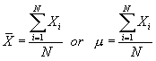
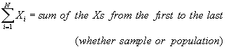
In this ranked distribution, the two middle scores are 3 and 4. If we add these two scores together (their sum equals 7) and divide the sum by 2, the median is 3.5. There are three scores below 3.5 (1, 2, and 3) and three scores above 3.5 (4, 4, and 5).

The mean is defined as the arithmetic average. It is the sum of all the scores in a distribution and that sum divided by the number of scores in a distribution.

Consider the following distribution:

To compute the mean for this distribution, we begin by adding the five terms. These five terms sum to 15. This sum is then divided by the number of terms in the distribution (in this case, 5). Hence, the mean for this distribution is 3.

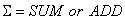
The mean is the first descriptive measure for which we actually have a formula:

	where:

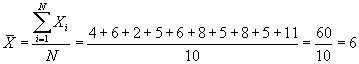
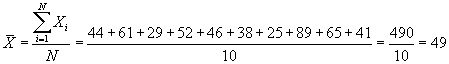
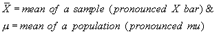
When computing the mean of a population, we label it with the Greek letter m (pronounced mu).

When computing the mean of a sample, we label it with the Latin letter X with a bar across the top (pronounced X bar).

While the formula for computing the mean is the same either for a population or sample, the use of different letters indicate whether the computed value is a parameter or a statistic.

Because the mean is such an important measure of central tendency, we want to consider additional examples. Consider the following two sample distributions. To compute the mean for each distribution, we sum the 10 scores and divide that sum by 10.

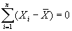
The mean has two important properties that set it apart from other measures of central tendency.

First, the sum of the deviations from a distribution's mean will always equal zero.

Written mathematically:

In other words, if we subtract the mean from every term in a distribution (creating deviations from the mean), these deviations they will always sum to zero.

Consider the following examples. For each of the three distributions (pictured below), the deviations from the mean sum to zero -- as the property indicates.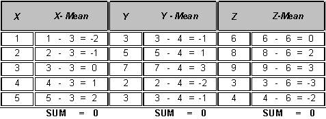

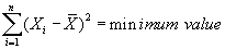
To demonstrate this important property, let's plot the deviations from the mean for our three distributions. The graphs clearly demonstrate that the sum of deviations ABOVE the mean is the same as the sum of deviations BELOW the mean.

The second property of the mean establishes that the sum of squared deviations from a distribution's mean will always equal a minimum value.

Written mathematically:

In other words, if we subtract the mean from every term in a distribution (creating the deviations from the mean), square these deviations, and then sum these squared deviations, the sum of squared deviations from the mean will always be the smallest possible sum of squared deviations. To illustrate, consider the following distribution (labeled X) whose mean is 3. First, we compute the squared deviations from the mean. Second, we compute the squared deviations from the constant 4. Third, we compute the squared deviations from the constant 2.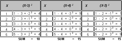

In the first set of columns, we've computed the sum of squared deviations from the mean. In the second set of columns, we've computed the sum of squared deviations from the constant 4. In the third set of columns, we've computed the sum of squared deviations from the constant 2.

While the sum of squared deviations from the mean equals 10, the sum of squared deviations from the constants 4 and 2 equals 15. In other words, the sum of squared deviations from the mean is SMALLER than the sum of squared deviations from the either the constant 4 or 2.

You should take the time to confirm this property for yourself. You might, for example, subtract a constant of one from every term in the distribution. If you do, you will verify that the sum of squared deviations from the mean is SMALLER than the sum of squared deviations from the constant one.

At the moment, this property of the mean appears rather useless. And while it is true this property has no immediate value for us, its value will become apparent in later units.

While all three of these measures of Central Tendency describe the middle or center or typical score within a distribution, they are different in many ways.

First, the mode is the crudest measure of central tendency as it is affected by only one score within a distribution -- i.e. the score that occurs most often.

Likewise, the median is affected by only one score -- i.e. the middle score within a distribution.

In marked contrast, the mean is the most sensitive measure of central tendency, as all scores within a distribution affect its magnitude.

Consider the following two distributions:

Below are the measures of central tendency computed for each distribution:

Interestingly, the mode does not change from Distribution 1 to Distribution 2 -- despite the addition of a single large score -- confirming its rather crude nature. Likewise, the median changes very little -- from 2.5 to 3. But the mean or arithmetic average changes significantly -- confirming that the mean is sensitive to all scores in a distribution. In fact, the mean is literally pulled in the direction of the extreme score in Distribution 2. Let's demonstrate this with a graph.

The graphs below plot the data values in Distributions 1 and 2. For each plot, the mean is positioned across the graph.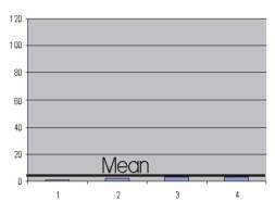

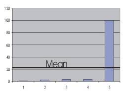
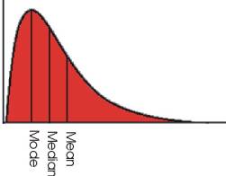
Notice that when a score of 100 is added to the second distribution, the mean is literally pulled in the direction of this larger score -- moving from a value of 2.25 in Distribution 1 to a value of 21.8 in Distribution 2.

The significant change in the value of the mean for Distributions 1 and 2 confirms the mean's sensitivity to all scores. However, this level of sensitivity is not always an advantage. Let's see why.

One important consideration in choosing a measure of central tendency is the shape of a distribution. Perhaps the most familiar shape of a distribution is the symmetrical distribution (or bell-shaped curve). If a distribution is symmetrical, the mean, median, and mode are equal or approximately equal in value.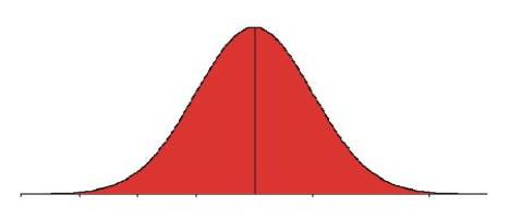

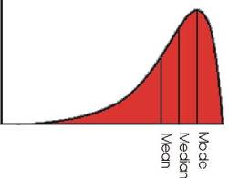
Mean=Median=Mode

Recall, the mode is the most frequently occurring score. Hence, the mode would occur where the distribution peaks -- in this case, the center.

The median is the middle score or the score that divides the distribution into two equal halves. Because the normal curve is symmetrical (one half is identical to the other half), the median also falls in the center.

Recall, the mean is the balance point of a distribution. If the distribution is symmetrical, the point where the distribution perfectly balances will also be the center.

But not all data distributions are symmetrical. When data distributions contain extreme scores, these distributions are described as skewed. Skewness describes the extent to which a distribution is asymmetrical about its mean.

A distribution is characterized as skewed when scores are concentrated on one end of the distribution's range with a tail forming on the other end of the range. Because scores can concentrate on either end of a distribution's range, distributions may be positively skewed or negatively skewed.

Positively Skewed Distribution (Skewed to the Right)

A distribution is positively skewed when it there is a clustering of numbers in the low end of the distribution and a tail extends towards the larger numbers (i.e. to the right). In positively skewed distributions, the mean is pulled to the right -- in the direction of the larger scores.

Mean > Median > Mode

A distribution is negatively skewed when there is a clustering of numbers in the high end of the distribution and a tail extends towards the smaller numbers (i.e. to the left). In negatively skewed distributions, the mean is pulled to the left -- in the direction of the smaller scores.

Mean < Median < Mode

In either case (positively or negatively skewed distributions), the mean is not usually the preferred measure of central tendency. Let's demonstrate with an example.

Income as a Skewed Distribution

A good example of a positively skewed distribution in the United States is income. The mean income in this country is considerably higher than the mode or the median. This is because there are a number of individuals with extremely large incomes -- Bill Gates, Paul Allen, Donald Trump, Ross Perot, Oprah Winfrey, etc. And, as we have already learned, the mean is pulled in the direction of these large incomes.

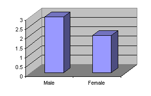
If we were to use the mean income to represent "typical income" in this country, the majority of individuals would have incomes BELOW the mean. Why? When a distribution is positively skewed, the mean is the largest measure of central tendency; the mode is the smallest measure of centraltendency; and the median falls between these two measures. Remember, the mean is pulled in the direction of the extreme incomes -- thereby greatly increasing its magnitude. On the other hand, the mode is the high point on the distribution, and in a positively skewed distribution of incomes, the high point falls on the low side. Regardless of the distribution's shape, the median remains the point that divides the distribution into two equal halves -- making it a true "middle" even for any distribution. The mean's sensitivity to extreme values ensures that it will be larger than either the mode or median in a positively skewed distribution. On the other hand, the mode may actually be too small in value -- thereby underestimating the distribution's center. But with the median representing the true middle with 50 percent of the incomes below it and 50 percent of the incomes above it, we can be fairly certain we are getting an accurate picture of a distribution's middle. This stability across all distribution shapes makes the median a better choice for central tendency when a distribution is heavily skewed.

In short, when a distribution is positively skewed, the mode presents a less prosperous picture of income earnings and the mean presents a more prosperous picture of income earnings for individuals in this country. However, the median presents the most accurate picture of income earnings.

We also use Levels of Measurement to determine the appropriate measure(s) of central tendency. As we shall see, the relationship between measurement level and central tendency will also serve to focus our choices.

Recall, at the nominal level of measurement we have no underlying mathematical properties. Hence, neither the median nor the mean can be used with nominal level variables, as both of these measures require mathematical properties.

However, we can use the mode with nominal level variables. Consider the following example:

Sex Male Male Male Female Female

In this distribution, we have 3 males and 2 females. Hence the modal sex is male -- i.e. the sex that occurs most often.

With ordinal level variables, it is possible to use both the mode and the median. As already indicated, the mode is the most frequently occurring score. Consider the following example:

In this distribution, the modal response to the question "How happy are you?" is "very happy."

Likewise, we can identify the median response or the middle response by ordering the distribution. Note our distribution is already ordered from happy to unhappy and the median response is "very happy."

With Interval/Ratio level variables, it is possible to use the mode, median, and the mean. A good example of an interval/ratio variable is income. Consider the following distribution:

The following table summarizes the relationship between central tendency, distribution shape, and levels of measurement -- with the preferred measures listed.

Remember to consider both distribution shape and measurement level when choosing the appropriate measure of central tendency.

?

?

?

?

?